Learn how to freeze a row in Excel on Mahadees.com and unlock the power of efficient data management. Freezing rows is a fundamental skill for anyone working with spreadsheets. By freezing the top row, you can keep important headers in view while navigating through extensive datasets, making it easier to understand and analyze your information.
Our step-by-step guide on ‘how to freeze a row in Excel’ will empower you to save time, improve organization, and boost your Excel proficiency. Whether you’re a beginner or an experienced user, mastering this technique is essential for smooth data handling. Explore Mahadees.com today to discover expert insights and tutorials on Excel and other productivity tools!
Related: HOW TO RECALL AN EMAIL IN OUTLOOK
Table of Contents
YouTube Video: How to Freeze a Row in Excel
To make it very convenient for you we have created a YouTube Video on how to freeze a row in Excel. Please click the above link, have a look, and be sure to subscribe.
Related Video: YouTube Video on How to Recall an Email in Outlook
How to Freeze a Row in Excel
1. Open Excel in your PC
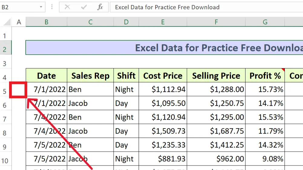
2. Now, select the cell that is below the row you want to freeze in first column
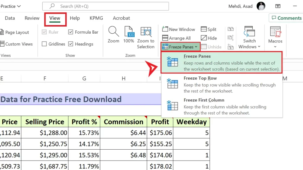
3. Go to view tab, click on freeze panes and select first option Freeze Panes
4. That’s it, you did it. ✅
Steps: How to Freeze a Row in Excel
Step 1: Selecting Cell
This step is crucial to understand how you can freeze a row in Excel. Your active cell should be exactly below the row you want to freeze and be sure that the active cell is in the first column otherwise your columns will also be frozen.
Step 2: Freezing Pane
When the relevant cell is active simply go to the view tab, click on freeze panes and there a drop down will appear. Click on freeze panes. Here you go!
View tab → Freeze panes → Freeze Panes
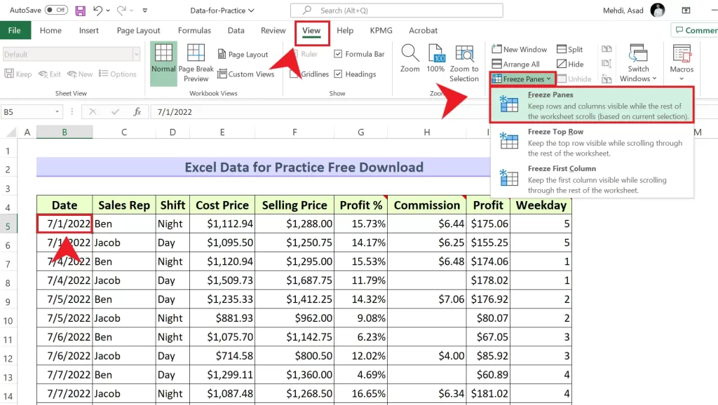
How to Freeze a Row and a Column
Freezing the row and column at the same time is the same as freezing the row but the only difference is cell selection. You need to select the cell that is below the row you want to freeze and after the column you want to freeze as shown below. Suppose I want to freeze column A and Row 4. I will select the cell B5. Go to the view tab —> freeze panes —> Freeze Panes.
That’s it.
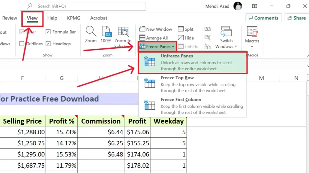
How to Unfreeze Panes
Now, you have learned how to freeze a row and column. To unfreeze the panes simply Go to the view tab, click on freeze panes and select the first option unfreeze Panes.
Conclusion
In conclusion, mastering the art of freezing rows in Excel is a crucial skill that can greatly enhance your efficiency and productivity when working with spreadsheets. As we’ve explored in this comprehensive guide on Mahadees.com, the process is simple yet immensely valuable for maintaining context and improving your data analysis experience.
By implementing the techniques and tips discussed here, you can effortlessly keep your headers visible while scrolling through extensive datasets, ensuring that you always have a clear overview of your information.
So, whether you’re a seasoned professional or just starting your Excel journey, freezing rows is a game-changer that can streamline your workflow and help you excel in your data management tasks. For more insightful Excel tutorials and valuable tips, be sure to explore our blog at Mahadees.com and stay ahead in the world of data manipulation.
Related: HOW TO ADD A SIGNATURE IN OUTLOOK

It¦s actually a cool and useful piece of info. I am satisfied that you just shared this helpful information with us. Please stay us up to date like this. Thank you for sharing.